claudia keuss
Urban Open Data
Card Game
Python | Datawrapper | Open Data
December 2024
Scripts for a fun, educational card game using Berlin’s open data, promoting awareness on urban topics and open knowledge.
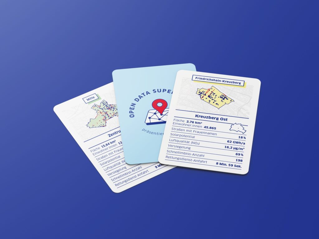
During my internship at the Open Data Informationsstelle (Technologiestiftung Berlin) in 2024, I contributed to the development of Open Data Supertrumpf, an analog data project inspired by the classic Top Trumps card game. Each card represents one of Berlin’s 58 administrative areas, using open datasets to compare various characteristics. For example, the ‘Air Quality’ category highlights where you can find the freshest air in Berlin, while ‘Fast Food Stalls’ reveals the districts with the highest density of döner and currywurst options. The ‘Female Street Names’ category sheds light on the presence (or lack) of streets named after notable women. All datasets used in this project are openly accessible, sourced from platforms such as the Berlin Open Data Portal and GDI Berlin.
My main responsibility was processing data for the six categories featured on each card. This project deepened my skills in data exploration, particularly working with geospatial data in Python and visualizing insights with Datawrapper. I also gained valuable insights and best practices from my colleagues. You can visit the GitHub page to learn more about the development of the game and its contributors. For additional insights into the process, check out the corresponding blog post [in German].
Process overview:
In order to understand the local differences in Berlin with regard to the various categories, we decided to aggregate the values at administration area level. All datasets contain spatial information, either as predefined LOR values – a spatial unit used for planning, forecasting, and monitoring demographic and social developments in Berlin – or as geographic coordinates. When spatial information was provided as longitude and latitude coordinates in a designated “geometry” column but lacked direct administrative area assignments, the spatial overlap was analyzed to determine their corresponding areas. This allowed for data aggregation by administrative area and enabled cartographic visualization.
In the following code block you will find a generalized approach based on the example of processing the ‘female street names’ dataset. While the approach may vary depending on the data source, it highlights key principles for working with geographic data.
      # Libraries
import pandas as pd
import geopandas as gpd
import matplotlib.pyplot as plt

# Load geojson files
admin_areas = gpd.read_file("../data/raw/admin_area.json")
gdf_category = gpd.read_file("../data/raw/category.geojson")

# Data exploration
gdf_category.shape
print(gdf_category.isna().sum())
print(gdf_category.dtypes)
etc...

# Subset relevant categories
categories_of_interest = ["A", "B"]
gdf_filtered = gdf_category[gdf_category["category"].isin(categories_of_interest)]
print(gdf_filtered.head())

# Check for empty or invalid geometries
print(f"Empty geometries: {len(gdf_filtered[gdf_filtered.is_empty])}")
print(f"Invalid geometries: {len(gdf_filtered[~gdf_filtered.is_valid])}")

# Ensure consistent CRS
if admin_areas.crs != gdf_filtered.crs:
    gdf_filtered = gdf_filtered.to_crs(admin_areas.crs)

# Plot data
fig, ax = plt.subplots(figsize=(10, 10))
gdf_filtered[gdf_filtered["category"] == "A"].plot(ax=ax, color="red", label="Category A")
gdf_filtered[gdf_filtered["category"] == "B"].plot(ax=ax, color="blue", label="Category B")
plt.legend()
plt.show()

# Function to analyze spatial intersections
def count_category(admin_area, gdf_filtered, category):
    intersections = gdf_filtered[gdf_filtered.intersects(admin_area.geometry)]
    unique_count = intersections[intersections["category"] == category]["name"].nunique()
    print(f"Admin Area: {admin_area['name']}, Unique_{category}: {unique_count}")
    return unique_count

# Apply functions to admin areas
admin_areas["unique_A"] = admin_areas.apply(lambda row: count_category(row, gdf_filtered, "A"), axis=1)
admin_areas["unique_B"] = admin_areas.apply(lambda row: count_category(row, gdf_filtered, "B"), axis=1)

# Subset final dataset
final_df = admin_areas[["id", "name", "unique_A", "unique_B"]]
print(final_df.head())
Please contact the ODIS team if you are interested in the card game.