claudia keuss
Housing Affordability
Python | EDA | (Un-)Supervised Learning
March 2024
This data analysis project aims to provide insight into the various factors influencing the medium value of owner-occupied homes (MEDV) in Boston. The medium value is an indicator for housing affordability.
The data for this analysis is sourced from the StatLib-Archive of Carnegie Mellon University and contains 506 entries, with each entry describing a suburb in Boston. It was originally published in 1978 by Harrison, D. and Rubinfeld, D.L. in “Hedonic prices and the demand for clean air“.
The analysis focuses on variables such as:
- per capita crime rate by town (CRIM),
- average number of rooms per dwelling (RM),
- weighted distances to five Boston employment centres (DIS)
- percentage of lower status of the population (LSTAT)
- medium-value of owner-occupied homes in $1000s (MEDV)
..and examines the following key questions:
- Which variables have the greatest influence on MEDV?
- Which variables correlate positively and which negatively with MEDV?
- To what extent do the districts differ? What are the key separating features?

Exploratory Data Analysis & (Un-)Supervised Learning Models
This analysis explores patterns and predictive modeling in the dataset using a combination of statistical and machine learning techniques. It begins with a correlation analysis to identify relationships between the variables, followed by scatter plots for visual insights. Unsupervised learning is applied using K-Means clustering to uncover hidden patterns. Next, predictive modeling is performed with supervised learning methods, including Multiple Linear Regression, K-Nearest Neighbors, Decision Tree, and Feedforward Neural Network, to evaluate different approaches for making accurate predictions of MEDV.
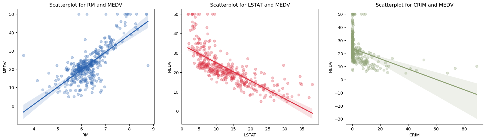
Correlation
Unsupervised learning model:
K-Means clustering
K-Means clustering
ØMEDV= 13.398851 (in $1000s)
Cluster 3: 7 data points
ØMEDV= 8.528571 (in $1000s)
% lower status vs. crime rate
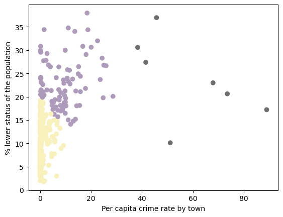
The first scatterplot illustrates the relationship between low-status population proportion and crime rate per capita. Cluster 2 has a low crime rate (up to 10%) and a low proportion of low-status residents (2–20%). Cluster 1 is more varied, with one or both values higher. Cluster 3, consisting of seven data points, shows a high crime rate (38–95%) and a broader range (10–40%) of lower-status population, though areas with high crime and a relatively small low-status population appear to be exceptions.
distance to employment centers vs. % lower status
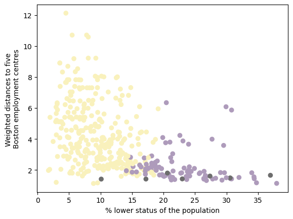
The second scatterplot depicts the relationship between low-status population proportion and distance to five Boston employment centers. Cluster 3 has consistently short distances but a wide range (10–37%) of low-status residents. Cluster 2, with the lowest crime rate and up to 20% low-status population, is spread both near and far from employment centers. Cluster 1 is mostly near employment centers, occasionally at medium distances, and has a relatively high low-status population (15–40%).
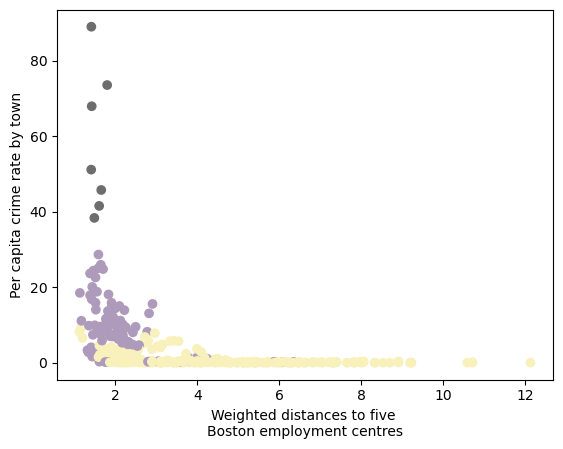
crime rate vs. distance to employment centers
Supervised learning models:
Multiple Linear Regression, K-Nearest Neighbors, Decision Tree, Feedforward Neural Network
1. Multiple Linear Regression
A multiple linear regression is used to predict MEDV (Median value of owner-occupied homes) based on features like LSTAT, RM and DIS. After dividing the data into training and test data, initialization and training the model the regression model is evaluated using the mean squared error (MSE) and R² score.
Results of the analysis:
Mean squared error: 0.018198038881035886
R²: 0.5630991043919185
Regression coefficients:[-0.50965825 0.59985805 -0.04213567]
2. K-Nearest Neighbors
The K-Nearest Neighbors (KNN) algorithm is used to predict MEDV based on the features LSTAT, RM and DIS. For this analysis I defined a model that looks at five neigbours when predicting MEDV and used the ball tree algorithm and the euclidean distance to measure similarities between the median value of owner-occupied homes. Since this is a regression task that involves predicting a continuous target variable (MEDV), the KNeighborsRegressor (instead of KNeighborsClassifier) is an appropriate choice, as it estimates values based on the average of the nearest neighbors. The performance of the model is again evaluated by the mean squared error and R² score.
3. Decision Tree
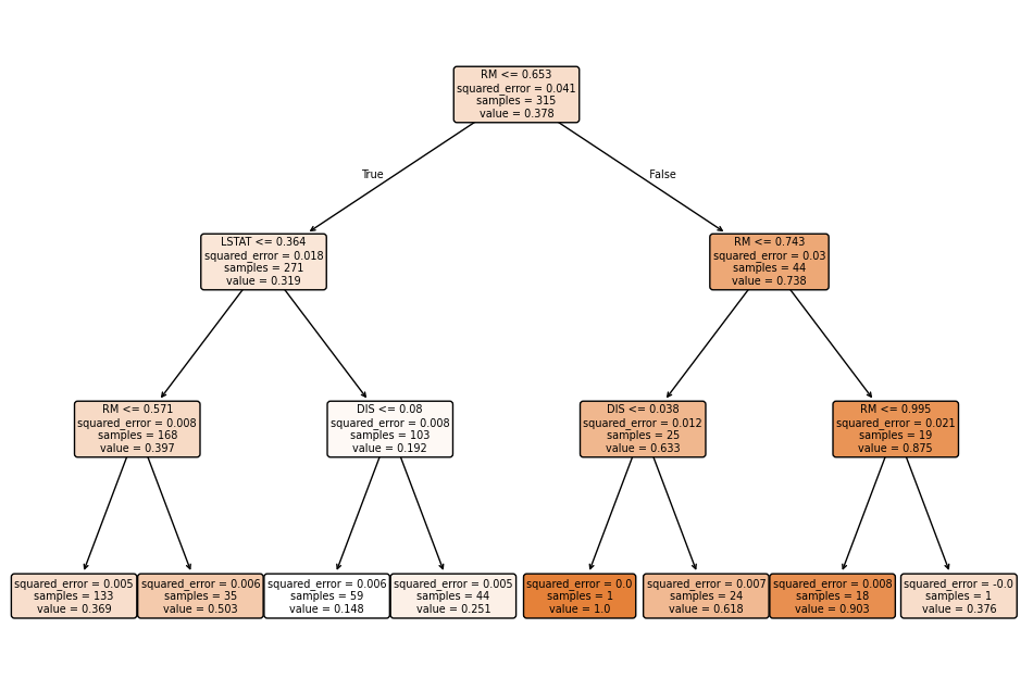
A Decision Tree splits the data into different groups based on certain conditions (or features) that maximize prediction accuracy. The division of the data follows the feature that enables the best separation of the data (here: RM). This is done by selecting the feature and threshold that provide the greatest purity or information gain.
4. Feedforward Neural Network
A Feedforward Neural Network (FNN) is used to predict MEDV based on the features LSTAT, RM and DIS. The following code demonstrates the process of building and training a FNN using PyTorch for regression. First, the input features (LSTAT, RM, DIS) and the target label (MEDV) are converted into tensors using the torch library. The data is then split into training (80%) and testing (20%) sets. The neural network (NN) is defined using the Net class, which consists of three layers: an input layer, a hidden layer, and an output layer. The ReLU activation function is used in the hidden layer and allows the network to learn and model complex, non-linear relationships in the data. During training, the Adam optimizer adjusts the model’s weights to minimize the loss. After training, the model’s performance is evaluated using the mean squared error (MSE) and R² score to compare the predicted outputs with the actual values. The training process involves multiple epochs to refine the model’s accuracy.
Results of the analysis:
Mean Squared Error: 0.0059572247315634675
R²: 0.8537254044419185
      # features= input data/ predictors = LSTAT/RM/DIS
# target = target variable/ dependent variable = MEDV

# convert into tensors
inputs = torch.tensor(X_train.values, dtype=torch.float32)
labels = torch.tensor(y_train.values, dtype=torch.float32).reshape(-1, 1)

# Division of the data set into training and test data
train_size = int(0.8 * len(inputs))
test_size = len(inputs) - train_size


# The NN_ReLU class inherits properties from nn.Module
class Net(nn.Module):
    def __init__(self, input_size, output_size):
        #super()-methode executes the heritage
        super(Net, self).__init__()
        self.fc1 = nn.Linear(input_size, 300)
        self.relu = nn.ReLU()
        self.fc2 = nn.Linear(300, output_size)

    def forward(self, x):
        x = self.fc1(x)
        x = self.relu(x)
        x = self.fc2(x)
        return x


# Hyperparameter
input_size = 3 #Number of features/dependent variables, LSTAT/RM/DIS
output_size = 1 #one neuron for the result MEDV
learning_rate = 0.0001
num_epochs = 100

#Initializing the neural network
model = Net(input_size, output_size)

# loss function and optimization
lossFunc = nn.MSELoss()  # Mean Squared Error
optimizer = optim.Adam(model.parameters(), lr= learning_rate)

# Training of the neural network
for epoch in range(num_epochs):
    for idx, element in enumerate(inputs):

        # forward propagation
        outputs = model(element)
        loss = lossFunc(outputs, labels[idx])

        # Backpropagation and optimization
        optimizer.zero_grad()
        loss.backward()
        optimizer.step()

        if epoch % 10 ==0:
            loss_value = loss.item()
            current = idx * len(inputs)
            print(f"Epoch {epoch + 1}/{num_epochs}, Loss: {loss_value}, Batch: {current}/{len(inputs)}")

# Evaluation of performance
predicted_labels = [output.item() for output in model(inputs)]
mse = mean_squared_error(labels, predicted_labels)
print(f"Mean Squared Error: {mse}")

r2 = r2_score(labels, predicted_labels)
print("R²:", r2)
A FFN is one of the simplest types of neural networks and is primarily used for tasks such as classification, regression, and pattern recognition. In classification tasks the output is typically a set of probabilities for each class. In regression tasks the output is a single continuous value.
Insights from the analysis:
- The average number of rooms per apartment appears to be the feature with the greatest influence on the MEDV followed by LSTAT and lastly DIS.
- A high percentage of low-status residents (LSTAT) correlates most negatively and the number of rooms per apartment most positively with MEDV.
- Areas with a lower proportion of low-status population (Cluster 2) tend to have consistently lower crime rates.
- Cluster 3, which has the highest crime rates, is concentrated near employment centers, suggesting that crime might be more prevalent in urban centers.
- Cluster 2 (with the lowest crime and a relatively low proportion of low-status residents) is spread across different distances, indicating that economic opportunities aren’t necessarily tied to proximity to employment centers.
- Cluster 1 is more mixed, with some areas near employment centers still having a relatively high percentage of low-status residents.
Which model seems to be best suited for predicting MEDV?
- For example, I had initially scaled the data with the StandardScaler() for a z-standardization; however, after testing the MinMaxScaler(), it turned out that this scaling results in significantly better predictions.
- In terms of the K-Nearest Neighbors algorithm, other k values could be checked and a different metric used to calculate the distance. An algorithm other than the ball tree could also be tested.
- For the decision tree, a different maximum depth could be checked, among other things, although too many levels could cause overfitting.
- In the Neural Network, changes in the number of hidden nodes and in the choice of activation and optimization function could lead to improved performance.
- The number of epochs also has an impact on performance, and saving the model and subsequent retraining, could increase the number of correctly predicted data.